Manual for the graphical calculator:
TOPCALCULATOR

MENU

File

Open : Chooses the text file that you want to open in the notebook. (extension =. txt)

Save : Saves the file. (extension =. txt)

Print Notebook -> prints the notebook.

: Chart -> prints the graph.

Close : Closes the program.

Edit

Copy : Copies the selected text or graphics to the clipboard.

Cut : Cuts the selected text and stores it in the clipboard.

Paste : Pastes the text from the clipboard into the document

at the position of the cursor.

Tables

Open : Opens the f, g and h-tables..

Print : Prints a table.

Models

Models : Opens the model menu.

Settings

Settings : Opens the settings menu .

Extra

Video measuring : Plotting diagrams using a video movie (*.avi).

OVERVIEW

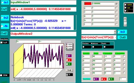
Buttons

In1 : Performs the calculation of InputWindow1. The outcome appears in OutputWindow1.
In2 : Performs the calculation selected in the notebook . The outcome appears in OutputWindow2.
In3 : Performs the calculation of InputWindow2. The outcome appears in OutputWindow2.
N : Enlarge or reduce the notebook. In the notebook appear all the calculations.
Functions
fgh : Shows in a separate window imported functions.

Input panels

curve : Shows the input for curve fitting.IDH_0041

var : Shows the input for real variables (VarWindow). (Default setting)

z : Shows the input for complex variables.

Curve

Z

Vectors : Shows the input for vectors.
Matrices : Shows the input for matrices.
Charts : Shows the input for plotting graphs. First a table is calculated . Make a choice from f, g, or h.

(Automaticcally the integral of the function between the specified limits is calculated; intf(….)= )

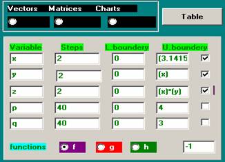
Charts panel

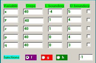
Variables : Enter here the function variables. When
a variable is checked, the button Table appears.

Press the button.

Steps : Type here the number of points, which should be calculated.
The default is 40.

Lower limit : The lower limit of the variable.
Upper limit : The upper limit of the variable.

Button (Table) : Starts the calculation and writes the values
to the database tables. Choose f, g or h depending on the calculation of a f,

g or h function..

ß this figure indicates the index of the functions f, g, h.

-1 Means no index.

MatrixWindow

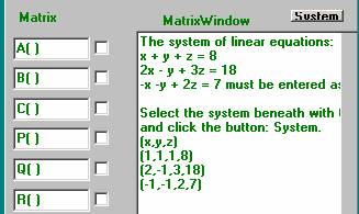
System : Solves a system of linear equations. This system must first be introduced in the matrix window according to the example. After entering the system, it should be selected with the mouse. Then click the button system.

Matrices have fixed symbols: A(), B (), C(), P(), Q(), R().
A matrix should be introduced according to the example into the matrix window. Then the matrix must be selected with the mouse. As a final step a matrix symbol must be checked.
Note: Each row must be started and completed with a hook.

VectorWindow

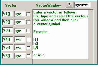
S: Solves a system of not linear equations. This system must first be introduced in vectorformat into the vectorwindow according to the example. After entering the system, it should be selected with the mouse. Next click on S.
Note: Variables in the vector coordinates should be introduced separately into the window beside S.

Vectors have fixed symbols: V1(), V2(), V3(), V4(), V5(), V6().
A vector should be introduced according to the examples into the vector window. Then the vector must be selected with the mouse. As a final step, a vector symbol must be clicked.
A vector coordinate is started and ended with a hook.

ChartWindow

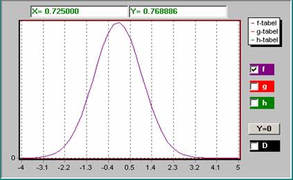
Buttons

f : Plots the graph from the f-table.
g : Plots the graph from the g-table.
h : Plots the graph from the h-table.

D : Plots with the depth chart.
3Dim : Plots a 3-dimensional graph.
Y = 0 : Calculates a zero point near the chosen coordinates.
The outcome appears in the notebook.

X-and Y-windows: By clicking on the chart with the left mouse button
the coordinates appear in these windows.

In / Out Zoom: With the left mouse button one can select a part of the graph
to enlarge it.
Functions f, g, h: Shows a list of all imported functions.

Calculations and formulas

Calculations and formulas can be introduced in three places.

1) In InputWindow1. Type the calculation or formula and click In1. The outcome appears in Out1.

2) In InputWindow3. Type the calculation or formula and click In3. The outcome appears in Out3.

3) In the notebook. Type the calculation or formula and then select it with the mouse and click In2. The outcome appears in Out2 and in the notebook.

Examples
As an example, invoervenster1.

1) Type 3 +5 * 7 / 9 = and click In1. The outcome appears in Out1.
     This is the same as 3 + (5 * 7) / 9 =

2) Type sin (4) = and click In1.

3) Type f (x) = (sin (x) + cos (x)) and click In1.
Next with f(number)= any function value can be calculated.

4) Type g (x) = (2 * (x) ^ 3 +1). The power operation is evaluated first.
This formula can also be introduced as g (x) = (2 * x ^ 3 + 1) without brackets around the variable within the function argument. g(number)= calculates any function value.

Notes to the examples 3 and 4.
a) Variables do not always have to be between brackets. See further under types of variables.
b) Functions are defined as follows: e. g. f (x) = (function definition)
or as f (x, y, z, u, v, w) = (function definition) to a maximum of 18 variables.
For functions the following symbols are available: f, g, h. From these functions
tables and graphs can be made.
Moreover, the symbols also available are : f0, f1,. . f9, g0, g1,. . g9, h0, h1,. . h9.
From these functions tables and graphs can be made by setting the function index in the
Chart window. See → ß this figure is the index indicated by the functions f, g, h (-1 Means no index)

An indexed function can also be assigned to f, g or h.
Example: g (x) = (f1 (x)) Also in this way a graph can be plotted from f1(x).
See further under Plotting Charts

Types of variables
There are 2 kinds of variables.
1) Variables existing of 1 letter e.g. x, y, z ,..., X, Y, Z. ..., etc. These variables can be used without brackets.
2) Variables existing of 1 letter and an index of figures e.g. x001, x002, x003, etc. . These variables must be used with brackets, as (x001), (x002) etc.

Plotting charts

For the plotting of functions the following steps are necessary.
After a function e.g. f (x) = (sin (x)) has been introduced:

1) Click on Chart. (If not yet checked)
     A new panel appears where the data
     for the chart should be introduced.
2) Enter a lower and an upper limit.
3) Enter the number of steps (points). For example 40.
4) Click the checkbox at the right. There now appears a new button Table.
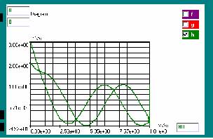
5) Click Table. If this button disappears the table for the chart is ready.
6) The graph is automatically drawn.

This will allow 3 charts simultaneously plotted for tables f, g and h.

Three-dimensional graphs

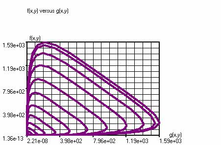
f(x,y)=(sin(x)+sin(y)+z) z=1

g(x,y)=(cos(x)-sin(y)+z) z=1

The above 2 graphs produce using Query the following chart, f(x,y) versus g(x,y).

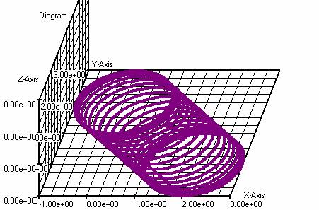
f (x, y) versus g (x, y) in the x-y plane.

The 3-Dim checkbox should be checked. Now a 3-D graphics window, a slider and 3 adjustable (x, y ,z) positions appear. With the slider, the position of the x-y plane against the Z-Axis can be varied. With the controls, the Zoom respectively the Shift along the 3 axes can be set. When clicked on the graph the X, Y, Z coordinates will appear at the top of the Chart window. This works best when the graph is plotted with separate points instead of an extended line (see Settings-> 3Dgraphics). In stead of the table values also the pixel coordinates can be displayed. This is easily done via Settings-> 3Dgraphics. When a function is available, the coordinates are calculated with this function. This is done automaticcally.

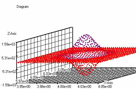
Example 3D Charts: The bivariate normal distributions: f (x, y) = ((5000/pi) * exp (-5000 * ((x-4) ^ 2 + (y-6) ^ 2))) and g ( x, y) = ((5000/pi) * exp (-5000 * ((x-4.02) ^ 2 + (y-6) ^ 2))) produce the following 3-dimensional graphs for x: 3.95 to 4.05 and y: 5.95 to 6.05.

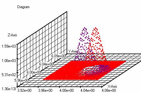
f(x,y)=((5000/pi)*exp(-5000*( (x-4)^2+(y-6)^2)))

g(x,y)=((5000/pi)*exp(-5000*( (x-4.02)^2+(y-6)^2)))

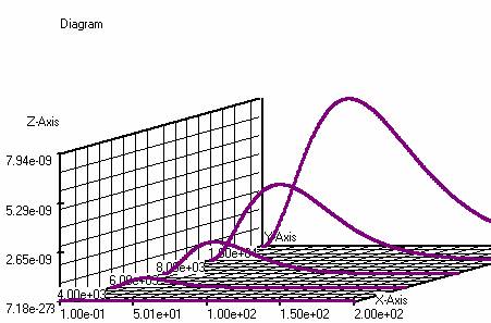
The above graphs produce, using Query, f (x, y) versus g (x, y)

f(x,y)=((5000/pi)*exp(-5000*( (x-4)^2+(y-6)^2))) (purple)

g(x,y)=((-5000/pi)*exp(-5000*( (x-4)^2+(y-6)^2))) (red)

Radiation curves of Planck.

f(f,T)=((6.1677E-13*((f)^3))/( exp( (4.7979E2*(f))/(T))-1))

f: (0.1-200) 400 steps, T: (2000-10000) 4 steps

Charts in the complex plane

Functions of a complex variable can be plotted in the 3-Dim graphs window.
The complex variable than should be split into a real part and an imaginary part.
E.g. f (z) = sin (z): z = x + j * y is complex, is introduced as follows: f (x, y) = sin (x'y) (Note the emphasis (x'y) to the top ). Now f (x, y) a complex function of the 2 real variables x and y, where x represents the real part and y the imaginary part. The variable panel should be set to “Var” and not to “Z”. See complex numbers for the introduction of a complex figure. The value of f (x, y) is saved as a complex number. Either the absolute value or the argument of f (x, y) is plotted in the complex plane, which can be established under "SettingsàGeneral”.

Parametric equations

1^e method

Using Structured Query Language (SQL) columns from various tables can be combined into a new table. Under the menu option Tables-> Query a SQL command can be entered.

Example: combination of 2 parametric equations.
(angles must be set to radians in the main under Settings / General.)

Enter: f(t)=(t+2*sin(2*t))

g(t)=(t+2*cos(5*t))

Using the standard command produces a table of f (t) versus g (t) by pressing the SQL START button.

Using To 3DIM-> On the table is sent to the 3DIM graphs window.

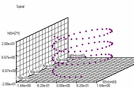
Application of SQL : Spiral

f(t)=(sin(t))

g(t)=(cos(t))

h(t)=(2*t)

Number of steps  : 100 ; t : -10 10 ; Angles in radians.

SQL Command:

select f_nr, f_functie, g_functie, h_functie from f_tabel.dbf, g_tabel.dbf, h_tabel.dbf where f_nr = g_nr and g_nr=h_nr;

2^e method

Using the menu option Models, graphs can be plotted based on parametric equations

Example

Program Startvalues

t=t+dt t=0

x=sin(2*(t))+0.5 dt=0.1

y=1.3*cos(t)+0.5 x=0.5

y=1.8

Note: Set angles to radians in the main menu under Settings/General.

Using matrices

Overall

Matrix data can only be introduced in the matrix window.
The matrix window appears when the matrix button is clicked. This button is next to the charts button.
In the matrix window it is shown how to introduce matrix data

After a matrix has been introduced matrix operations can be performed.
For example, operations on a matrix A().
These operations must be performed in an InputWindow.

Matrix operations

a) The inverse of a matrix A( ) , enter: A( )^-1

b) The transpone of a matrix A( ), enter: A( )^ Tr

c) Transformation of a tridiagonal matrix A() to a diagonal matrix : enter diag(A)

d) Transformation of a symmetric matrix A() to a tridiagonal matrix using the method

of Householder, enter : tridiag(A).

Matrix calculations.
a) The sum of the matrices A() and B(): enter A () + B () =
b) The subtraction of the matrices A() and B(): enter A() - B() =
c) The product of matrix A () and matrix B (): enter A() * B() =
d) The third power of matrix A(): enter A() ^ 3
e) A combination of operations and calculations: e.g. A() ^ -1 + B() * C() ^ 3 =

Matrix functions

For example f(x, y)=( 2*A( )^-1 + B( )^3 ) , where x en y are two variables that appear in A() en B().

These variables must be between brackets in the matrix.

Note: using matrix calculations and matrix functions arithmetic brackets are also allowed The order of operations inside the brackets is successively: exponentiation, multiplication, addition, subtraction.

The determinant of a symmetric matrix.

Using the following steps the determinant can be evaluated..

1) Enter the matrix in the matrix window.
2) Select the matrix and click on a matrix symbol (e.g. A()).
3) Type in an InputWindow det (A) =.

Eigenvalues en Eigenvectors of a matrix

The accuracy of the methods is adjustable in the settings menu under Iterations.

a) eigwn(A): Calculates all eigenvalues and eigenvectors of a matrix A(). The method is
   automatically selected. For symmetrical matrices: QR Method for non-symmetrical
   matrices: Inverse Power Method
b) eigwd(A): Calculates the dominant eigenvalue of a matrix A() according to the Power Method.
c) eigwds(A): Calculates the dominant eigenvalues of a symmetric matrix A() according to the
   Symmetric Power Method with fewer iterations than b).
d) eigwq(A, q): Calculates an approximate eigenvector and eigenvalue of a matrix A() in the neighborhood of
   q according to the Inverse Power Method. Successively performing this operation with
   the found eigenvalue as q, produces a more accurate eigenvalue.

Note: de maximum matrix size in this program is a 9 times 9 matrix.

Summation of functions

When summing a function, the function variable goes through a series of whole numbers from a starting value (a ) to an end value (b

Using the following command a function can be summed

a) For a function f(x) : type somf(x:a,b)=

a is : lower limit.

b is : upper limit .

b) For a function g(x) : type somg(x:a,b)=

a is : lower limit.

b is : upper limit

c) For a function h(x) : type somh(x:a,b)=

a is : lower limit.

b is : upper limit .

The definite integral of a function

There are two ways in which a function can be integrated.

1) When a table for a graph is made
the value of the integral appears automatically in the notebook.

2) By typing the following command in an InputWindow:

a) For a function f(x) : type intf(x:a,b)=

a is : lower limit.

b is : upper limit .

b) For a function g(x) : type intg(x:a,b)=

a is : lower limit.

b is : upper limit .

c) For a function h(x) : type inth(x:a,b)=

a is : lower limit.

b is : upper limit .

Multiple Integrals

Double and triple integrals can be calculated as well with fixed boundaries as with floating boundaries.
The order of integration is determined by the order of the variables in the VarWindow.
In the next example, this order is from top to bottom, y, x. (See also the example for triple integrals)
The order of the variables in the Chart Window is not important.

Double integral with fixed boundaries.

Example:

Integrates first over y and then over x.

Enter : f(x,y)=( (x) * (y)^2 )

Integration boundaries: x from 2.1 – 2.5 ; lower limit 2.1 , upper limit2.5.

y from 1.2 – 1.4 ; lower limit 1.2 , upper limit 1.4.

Number of steps for x and y is 4.

Integration method must be set on Composite Simpson. (See main menu : Settings)

Example of a triple integral
Integration method is Gauss. (See main menu: Settings)
Angles must be set to radians. 2 * pi = 6.283185.
(Integral of f (x, y, z) on a sphere using spherical coordinates)

Enter: f(x,y,z)=(5*cos(z)^2*(x)^2*sin(y)/((x)^4))

Number of steps for x and y and z is 6.

Integration boundaries: x from 1 – 2

y from 0 – pi

z from 0 -- 6.283185

In the notebook appears:

intf( x :1.000000,2.000000; y :0.000000,3.141593; z :0.000000,6.283185) 15.685618700000 Termen: 216

Integration with variable boundaries

In the Chart panel also variable boundaries can be filled in, in formula format. The order of integration is hereby determined by the order of the variables in the VarWindow. The following example shows this order from top till down nl. : z, y, x. (See VarWindow).

The order of the variables in the Chart panel is not of interest.

Example: triple integral with variable boundaries.

Integrates first over z, next over y and then over x.

VarWindow

Enter : f(x,y,z)=( 1/(y) * sin( (z) / (y) ) )

Integration boundaries x from 0 - p ; lower limit 0 , upper limit (3.1415926 ). Notice the brackets!

y from 0 – x ; lower limit 0 , upper limit (x) .

z from 0 – xy ; lower limit 0 , upper limit ((x)*(y)) .

Chart panel

Number of steps for x, y and z is 2.
Integration method is set to Gauss. (See Mainmenu: Settings à General)
Angles on Rad.

Integration of functions of complex variables

De integration method is by default Composite Simpson.

z is complex.

Examples

f(z)=( (z)^2)

Lower boundary : (0,0)

Upper boundary : (1,1)

Number of steps : 40

In the notebook appears:

intf( z :0.000000,1.000000) + j * intf( z :0.000000,1.000000) (-0.666667, 0.666667) Terms: 82

The outcome is : (-0.666667, 0.666667)

f(z)=cos(z)

pi= (3.141593, 0.000000)

Lower boundary is : (0, -3.141593)

Upper boundary is : (0, 3.141593)

Number of steps is : 40

In the notebook appears:

intf( z :0.000000,0.000000) + j * intf( z :-3.141593,3.141593) (0.000000, 23.097563) Terms: 42

The outcome is (0.000000, 23.097563)

Complex Contour Integration

The integration of a function of a complex variable z along a contour z (t) in the complex plane.
The complex variable and the contour should be introduced under main menu : Settings.
Likewise, the derivative z' of z to the parameter t should be introduced in the window dz under Settings in the mainmenu. The upper and lower limit of the parameter t have to be set in the chart panel.

Example:
f (z) = e ^ z / (z-2)
Enter: f (z) = (exp (z) / (z-2))
In the notebook appears:
f (z) = (exp (z) / ((z) -2)) (20.085537, 0.000000) z = (1.0,1.0)
The setup under main menu : Settings:
Contour = (p) + (r) * exp ((j) * (t)) z '= j * (r) * exp ((j) * (t)) (The contour is a round field at the point p)
In the VarWindow, (z): p = (2,0) r = (1,0)
In the Chart panel parameter t,: Lower boundary (0.0), Upper boundary: (6.283185,0)
In the notebook appears:
intf (t: 0.000000,6.283185) + j * intf (t: 0.000000,0.000000) (-0.000002, 46.426802) Terms: 42
Outcome: (-0.000002, 46.426802)

Example:
f (z) = (z-p) ^ m

if m=-1 and c=Contour around p in the complex plane.

if m is unequal -1 and c=Contour around p in the complex plane.

Enter: f (z) = ((z-p) ^ m), z = (1.0,1.0) p = (2.0,0.0) m = (5,0)

In the notebook appears:
f (z )=((( z) - (p)) ^ (m)) (1.000000, 0.000000) z = (1.0,1.0) p = (2.0,0.0) m = (5,0)

The setup under main menu : Settings:
Contour = (p) + (r) * exp ((j) * (t)) z '= j * (r) * exp ((j) * (t)) (The contour is a round field to the point p)

Integration boundaries for the parameter t, in the Chart panel: Lower boundary (0.0), Upper boundary: (6.283185, 0)
With r = (1.0,0.0) and m = (5,0) in the VarWindow (option z):

In the notebook appears:
intf (t: 0.000000,6.283185) + j * intf (t: 0.000000,0.000000) (0.000004, 0.000001) Terms: 42
Outcome: (0.000004, 0.000001)

m = (-1.0):
In the notebook appears:
intf (t: 0.000000,6.283185) + j * intf (t: 0.000000,0.000000) (0.000000, 6.283185) Terms: 42

Outcome: (0.000000, 6.283185)

Differentiation of functions

Note.: his only works with the function symbols f, g, h and not with indexed function symbols.

With the help of the following command a function e.g. f (x) can be differentiated

a) Determination of the first derivative of f(x).

Typ in an InputWindow: g(x)=(difxf(x))

Read this as “Differentiate (dif) to x (x) the function f(x)”.

b) Determination of the second derivative of f(x).

Typ in an InputWindow: h(x)=(difxxf(x)

Read this as “Differentiate (dif) two times to x (xx) the function f(x)”.

Note. The stepsize h for differentiating is adjustable.

Now graphs can be drawn simultaneously from f(x), g(x) and h(x) after tables have been made from these functions. The table settings should be the same for all three functions

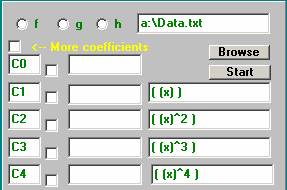
Curve fitting

On the right side of the VarWindow is the button for curve fitting (curve)

With the use of curve fitting a polynomial function can be determined from a series of number pairs. Curve fitting

With the use of curve fitting also interpolation and extrapolation can be performed.

The following steps are necessary.
1) Make a table with the measured values. This can be done in two ways.

a) On a diskette (a: drive).
  This file must have the following format:
Type in the first line: x y , next type under x the x-values and under y the y-values sepatated by spaces.
b) With the help of the tables f, g or h.
        These tables can be found in the main menu under tables.
Fill in a table.

2) Click the number of constants (C0, C1, C2 etc.) with which the polynomial function must be created.
3) Click on the button start.

Note. the polynomial function appears in InputWindow1 as g(x)=(….).

Non linear equations with one unknown

The functie solve( ) solves a non-linear equation according to the Muller method.

Example: (x)^3 - 2*(x)^2 - 5 = 0

Enter : f(x)=( (x)^3-2*(x)^2-5)

Note.: This only works with the function symbols f, g, h and not with indexed function symbols like f1(…)= etc.

(Find an approach of zero near the point x = 2.0)
Enter: solve (f, 2.0) =.
Or make a graph of the function f (x) = ((x) ^ 3-2 * (x) ^ 2-5) and hit a point in the vicinity of f(x) = 0.
Then press the button Y = 0.

In the notebook appears:
Iterations Muller method: 5 Zero approach:
solve (f, 2) = 2.690647 x = 2.690647
x = 2.690647 is the penultimate approach.

Non linear equation with a complex solution.

The function f (x) = (16 * (x) ^ * 4-40 (x) ^ 3 * 5 (x) ^ 2 20 * (x) +6) = 0 has two real and one complex solution.
Enter: f (x) = (16 * (x) ^ * 4-40 (x) ^ 3 * 5 (x) ^ 2 20 * (x) +6)
Note.: This only works with the function symbols f, g, h and not with indexed function symbols like f1(…)= etc.

Then, enter : solve (f, 2) =.
In the notebook appears:

Iterations Muller method: 4
Zero approach:
solve (f, 2) = 1.970446 x = 1.970446

Enter: solve (f, 1) =.
In the notebook appears:

Iterations Muller method: 5
Zero approach:
solve (f, 1) = 1.241677 x = 1.241678

Enter: solve (f, 0) =.
In the notebook appears:

This approach provides no real solution.
Click on z and enter the function as a complex function,
for a complex solution.

The complex function provides the following solution:
Iterations Muller method: 7
Approximate solution:
solve (f, 0) = (-0.356062, 0.162759) x = (-0.356061, 0.162758)

Systems of non linear equations

There are two ways to find a solution.
Method 1 looks first for an approximate .

Method 1:
Use the mouse to the example in the VectorWindow.
Then click S.
Angles must be set on Rad.

In the notebook appears:

Functions system
Vx = (3 * (x)-cos ((y) * (z)) -0.5)
Vy = ((x) ^ * 2-81 ((y) 0.1) ^ 2 + sin (z) +1.06)
Vz = (exp (- (x) * (y)) 20 * (z) + (10 * pi-3) / 3)

f1 (x, y, z) = (difxg (x, y, z))
f1 (x, y, z) = (difyg (x, y, z))
f1 (x, y, z) = (difzg (x, y, z))
  * * * * * *
Iterations SteepDescent method: 3
Approximate solution.
x = 1.122011e-02
y = 1.009712e-02
z =-5.228119e-01
   * * * * * * * * * * * * * * * * * * * *

   * * * * * * * * * * * * * * * * * * * *

   * *
Iterations Newton method: 5
x = 5.000000e-01
y = 4.339851e-10
z =-5.235988e-01

Method 2:
Use the mouse to select the example in the VectorWindow and click a vector symbol, e.g.V1().
With the help of the function solve (....) an approximate solution can be specified.
E.g.: solven (V1 (1,1,1)) =
Angles must be set on Rad..

In the notebook appears:

Vector V1
Vx = (3 * (x)-cos ((y) * (z)) -0.5)
Vy = ((x) ^ * 2-81 ((y) 0.1) ^ 2 + sin (z) +1.06)
Vz = (exp (- (x) * (y)) 20 * (z) + (10 * pi-3) / 3)

f1 (x, y, z) = (difxf (x, y, z))
f1 (x, y, z) = (difyf (x, y, z))
f1 (x, y, z) = (difzf (x, y, z))
  * * * * * * * * * * * * * * * * * * * * * *

   * * * * * * * * * * * * * * * * * * *
Iterations Newton method: 5
x = 5.000000e-01
y = 4.507480e-10
z =-5.235988e-01
solven (V1 (1,1,1)) = 0.000000 x = 0.500000 y = 0.000000 z = -0.523599 N = 1.0 h = 1.0

Systems of linear equations

In the MatrixWindow is shown how to enter a system of linear equations.

The number of unknowns has a maximum of 6.

By pressing the button "system" the system is resolved.

The solution appears at the bottom of the MatrixWindow.

Differential equations

Initial value probems.

Method of Euler.

Example:

Type f(x)=(y-x^2+1) and next euler(f(y0:0.5))=.

f(x)=(y-x^2+1) is identical to dy/dx=y-x^2+1 .

d? indicates that in the GraphicsWindow a variable must be entered with a starting and an end value In this example this variable is x. As a starting value of x we choose 0 and as end value we choose 2.0 The number steps is 10. De The starting value of the solution is : y0=0. 5. In table h appear the following values for y and x.

0.5 0

0.8 0.2

1. 092 0.4

1.36 0.6

1.588 0.8

1.76 1.0

1.86 1.2

1.872 1.4

1.78 1.6

1.568 1.8

1.22 2.0

Runge-Kutta method. (RK4)

Example:

Type f(x)=(y-x^2+1) and next rungek(f(y0:0.5))= .

Furthermore, we choose the same settings as in the method of Euler.

Runge-Kutta-Fehlberg method (RK45-method).

Example:

Type f(x)=(y-x^2+1) and next rungekf(f(y0:0.5))=.

Furthermore, we choose the same settings as in the method of Euler.

Systems of Differentialequations

The method used here is: Runge-Kutta method (RK4) or (RKF) without variable stepsize.
The general command for the RK method reads: rungeks (f1, f2 ,..., fn (Y1 :..., Y2 :...,...., Yn :...))=
Or for the RkF method: rungekfs (f1, f2 ,..., fn (Y1 :..., Y2 :...,....., Yn :...))=
The settings for the RKF method must be made under differential settings on the main menu.

Example 1

A system of two differential equations, n = 2.
Type and enter.
f1 (t, Y1, Y2) = (-4 * (Y1) 3 * (Y2) +6)
f2 (t, Y1, Y2) = (-2.4 * (Y1) 1.6 * (Y2) +3.6)
The starting values are, for Y1: 0 and Y2: 0.
and then type rungeks (f1, f2 (Y1: 0, Y2: 0) =

The integration variable is t. As a starting value of t we choose 0, and 0.5 as final value.
For the number of steps we choose 5.
The table letter is adjustable. (See Settings-> Solution Table Differential Equations)
In the table appear the values of Y1 and Y2. Under Function Y1 is tabulated and under Y, Y2 is tabulated.
In the GraphicsWindow appear the charts.

Example 2

n=2.

Type:

f1(x,Y1,Y2)=(-2*(Y1)+ (Y2)+2*sin(x))

f2(x,Y1,Y2)=((Y1)-2*(Y2)+2*(cos(x)-sin(x)))

and next; rungeks(f1,f2(Y1:2,Y2:3)=

The initial values are, for Y1: 2 en voor Y2: 3.

The integration variable is x. As a starting value of x we choose 0 and as a final value 10.
For the number of steps we choose 60. Angle x in radians.
In the GraphicsWindow appears the following solution for Y1 and Y2.

Butcher Matrix

Explicit methods with Butcher coefficients

Under SettingsàDifferentialequationsàButcher Matrix, the Butcher coefficients can be filled for an explicit Runge-Kutta method. Differential equations àUnder Settings
The corresponding command reads: rksbutcher(f1,f2,...,fn(Y1:...,Y2:...,....,Yn:...))=.

The settings are the same as for the above-described RK methods.
With the buttons f, g, h under ChartSettings the table can be chosen to store the solution.

Calculations with Vectors

Input of vectors. (See VectorWindow)

After a vector has been entered, operations on the vector can be performed.

For example operations on a vector V1().
These operations must be entered in an InputWindow.

Vector calculations.
a) The sum of the vectors V1 and V2: enter V1() + V () =
b) The subtraction of the vectors V1 and V2: enter V()-V2() =
c) The innerproduct of the vectors V1 and V2: enter V1(). V2() =
d) The outerproduct of the vectors V1 and V2: enter V1() * V2() =
e) The Jacobian of a system of equations: enter jac(V1()) =

Note. In calculations with vectors also arithmetic parentheses are allowed.
The sequence of operations (within the parentheses) is successively: exponentiation, outerproduct, innerproduct, addition, subtraction.

Vectors that contain variables can also be introduced as a function.
E.g. vector V1() contains:

Vx = (3 * (x)-cos ((y) * (z)) -0.5)
Vy = ((x) ^ * 2-81 ((y) 0.1) ^ 2 + sin (z) +1.06)
Vz = (exp (- (x) * (y)) 20 * (z) + (10 * pi-3) / 3)

Enter: f (x, y, z) = (V1 (x, y, z)), then using f (.., .., ..) = for each value of x, y and z the vector components can be evaluated.

Example: jacobian matrix:
Evaluation of the jacobian example of the system in the VectorWindow at the point x = 1, y = 1, z = 1.

First enter the coordinates x = 1, y = 1, z = 1 in the VarWindow.
Then select in the VectorWindow the example system and click on V1.
Then enter jac(V1()) = or jac (V1(1,1,1)) = in an InputWindow.
Angles must be set on Rad.

In the notebook appears:

Vector V1
Vx = (3 * (x)-cos ((y) * (z)) -0.5)
Vy = ((x) ^ * 2-81 ((y) 0.1) ^ 2 + sin (z) +1.06)
Vz = (exp (- (x) * (y)) 20 * (z) + (10 * pi-3) / 3)
f1 (x, y, z) = (difxf (x, y, z))
f1 (x, y, z) = (difyf (x, y, z))
f1 (x, y, z) = (difzf (x, y, z))
f1 (x, y, z) = (difxf (x, y, z))
f1 (x, y, z) = (difyf (x, y, z))
f1 (x, y, z) = (difzf (x, y, z))
f1 (x, y, z) = (difxf (x, y, z))
f1 (x, y, z) = (difyf (x, y, z))
f1 (x, y, z) = (difzf (x, y, z))
Jac (V1 ()) = Matrix U = 1.000000 x y z = 1.000000 = 1.000000 N = 1.0 h = 1.0

Matrix U (Output)
(3, 0.816573, 0.816573)
(2, -178.2, 0.524316)
(-0.354069, -0.354069, 20)

Vectorfields

a) Divergence of a vector at a point x, y, z : enter div (V ()) =
b) Rotation of a vector at a point x, y, z : enter rot (V1()) =
c) Gradient of a function f in a point x, y, z : enter grad(f (x, y, z)) =

Calculation of a gradient.
Note.: This only works with the symbols f, g, h and not with indexed variables.
Enter:
f (x, y, z) = (3 * (x)-cos ((y) * (z)) -0.5)
Angles on Rad!

Then: grad (f (1,2,3)) =
In the notebook appears:

f1 (x, y, z) = (difxf (x, y, z))
f1 (x, y, z) = (difyf (x, y, z))
f1 (x, y, z) = (difzf (x, y, z))
grad (f (1,2,3)) = Matrix U = 1.000000 x y z = 2.000000 = 3.000000 h = 1.0

Matrix U (Output)
(3)
(-0.065587)
(-0.374006)

Calculations with Complex numbers

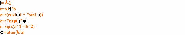
Complex numbers are entered as follows:

In the InputWindows 1, 2 and 3 as (a’b) or as

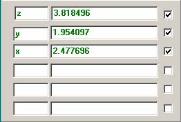
Note: In the VarWindow (z) for complex variables as (a, b).

Standard functions with complex numbers.

z has as format:

arg(z)

imag(z)

real(z)

abs(z)

sin(z)

sinh(z)

asin(z)

cos(z)

cosh(z)

acos(z)

tan(z)

tanh(z)

atan(z)

exp(z)

log(z)

ln(z)

sqrt(z)

Standard Formulas

General formulas

pi

sqrt(x)

(n)!

(n,m)! = n! / m(n-m)!

Trigonometric Formulas

For all angles : x in radians or in degrees (See Settings in the main menu)

sin(x)

asin(x)

sinh(x)

asinh(x)

cos(x)

acos(x)

cosh(x)

acosh(x)

tan(x)

atan(x)

tanh(x)

atanh(x)

Sa(x) : Sa(x)=sin(x)/x

Exponential and logarithmic Formulas

exp(x)

log(x)

ln(x)

Integral Functions

An example of an integral function is Si (x).
Si(x) is the integral of 0 to x of the function sin (x) / (x).
Si(x) = (sin(x) / (x)) is the so-called sample function. To obtain a graph enter: f (x, y) = (int (Sa (x))), together with the following settings. Angles must be set to radians. Si (x) converges to ± п / 2.  

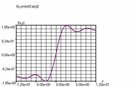
ChartWindow :

Variable Steps Lower boundary Upper boundary

x 40 0 (y)

y 40 -12 12

Note. : In the VarWindow x must be above y  ; x is the help variable, x runs from 0 to y.

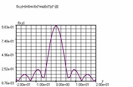
Fourier Integral

f(x,y)=(int(rect(x)*exp((x)*(y)*-j)))

This function calculates the Fourier integral of the rectangular pulse rect(x) with amplitude 1.

Settings in the ChartWindow:

Variable Steps Lower boundary Upper boundary

x 20 0 1

y 40 -20 20

Note. : In the VarWindow x must be above y  ; x is the running variable, x runs from 0 to y.

In the diagram, the absolute value of the complex outcome f (x, y) is shown.

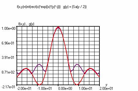
The above chart is the analog solution (g(y) = (Sa(y / 2)), (angles in radians) of the Fourier integral of rect(x) together with the numerical solution f(x, y).
Purple: f (x, y).
Red: g (y)

Periodic Functions (square and ramp)

Under Settings-> Periodic functions, for a square rect(x) and a triangle tri(x) using T1 and T2 the pulse duration can be set. Shift shifts the starting point of the graph compared to the origin.

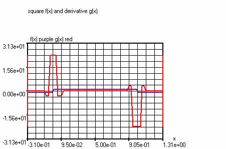
Example 1:

f(x)=(2*rect(x)-1)  (Square)

g(x)=(difxf(x))  (derivative of the sqare)

Under functions fgh appears the underlying formula for the derivative.

g(x)=((f(((x)-2*(h)))+$(((x)+2*(h)))-8*f(((x)-(h)))+$(((x)+(h)))+8*f(((x)+(h)))+$(((x)-(h)))-f(((x)+2*(h)))+$(((x)-2*(h))))/(12*(h)))

Chart panel

x: -4.0 – 5.0

Steps: 400

VariableWindow

h=0.05

SettingàPeriodic functions

T1=1.0

T2=1.0

Shift=-4.0

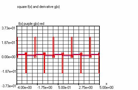
Example 2: Square and derivative.

f(x)=(2*rect(x)-1) 

g(x)=(difxf(x)) 

ChartWindow

x: -4.0 – 5.0

Steps: 4000

VariableWindow

h=0.005

SettingsàPeriodic functions

T1=1.0

T2=1.0

Shift=-4.0

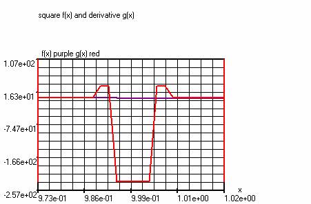
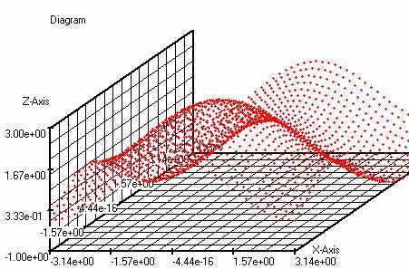
The above chart shows one negative slope(purple) of f(x)=(2*rect(x)-1)  and its derivative g(x) (red).

Primitivation

Example 1

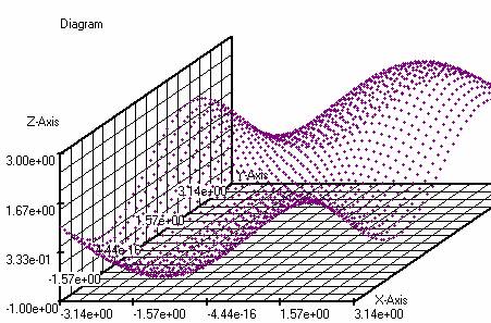
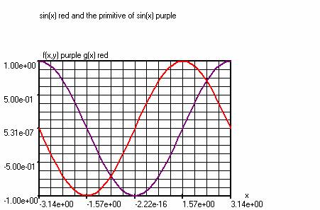
The primitive of sin(x) is -cos(x) + Constant

Using the command f (x, y) = (int (sin (y))), where the y variable is the running variable, we can draw the chart from the primitive of sin (x) and create the table of the primitive of sin (x)

 Red :  g(x)=(sin(x))

Purple :  f(x,y)=(int(sin(y)))

 Note. In the VarWindow,  the running variable y must be placed above the variable x.

                Steps Lower boundary         Upper boundary

x :            40                           -pi                           +pi

y :           40                           -1.570796               (x)

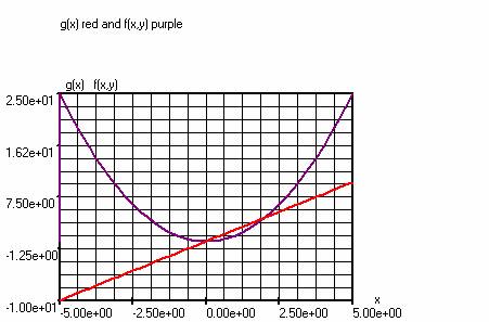
Example 2

The primitive of g(x)=(2*(x)) is entered as follows:

f(x,y)=(int(2*(y))),. y is the running variable.

Note. In the VarWindow the running variable y must be placed above the variable x.

 ChartWindow :

                Steps Lower boundary Upper boundary

y :           40                           0                             (x)

x :            40                           -5.0                         +5.0